ITALY COVID-19 DATA ANALYSIS (by Max Pierini)
Stima downloads dell'app Immuni (vedere link per il metodo utilizzato).

info@maxpierini.it
In this jupyter notebook, we'll analyse italian COVID-19 data gathered from Dipartimento di Protezione Civile GitHub repository (link).
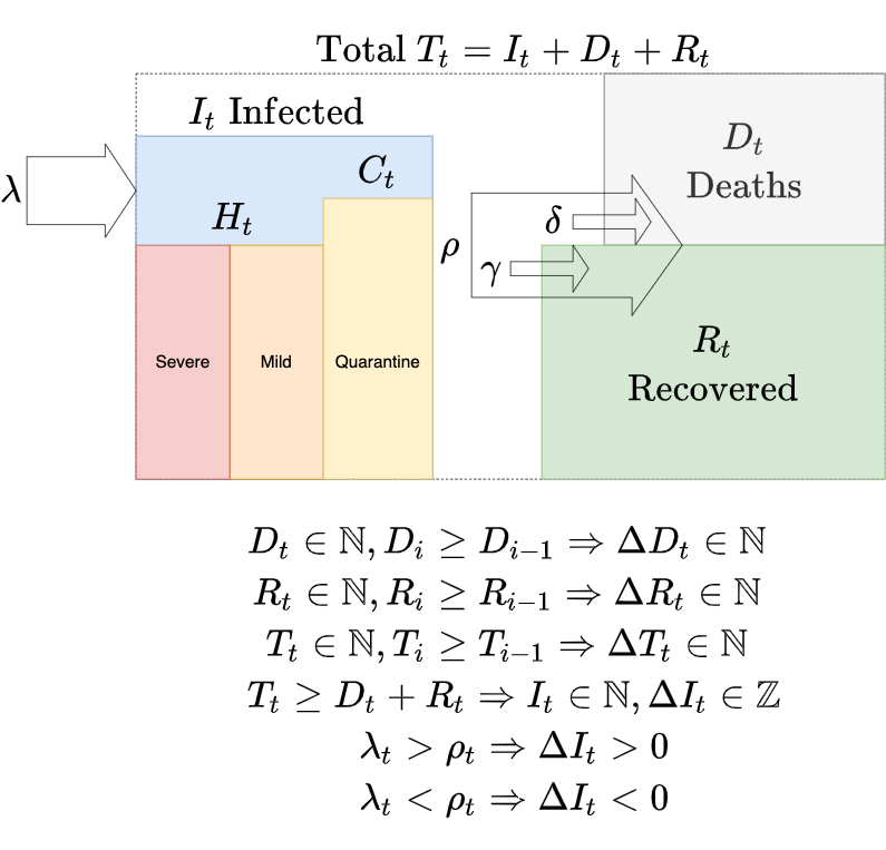
We'll consider following compartments
- R recovered (total cumulative recovered cases)
- D deaths (total cumulative deaths caused by COVID-19)
- T confirmed (total cumulative cases)
- infected + recovered + deaths
- I infected (current positive cases)
- confirmed - (recovered + deaths)
- H hospitalized + C quarantine, where hospitalized can ben mild or severe (intensive care)
ITALY TABLE OF CONTENTS
Daily variations
Percentages & Rates
Extra
TEST
Other plots on this website:
- NEW! Italy predictions
- Italy (nation)
- Italy (regions overview)
- Italy (regions single)
- Italy (province overview)
Also on this website:
and get the most recently updated data from D.P.C. GitHub Repository, loading them into a dictionary.
Let's check the dates of the downloaded data:
Smoothed daily variations
And finally take a look to the complete result, hiding original data, flexes and vertical lines:
PERCENTAGE VARIATIONS
MORTALITY & RECOVERY RATES
!!! PLEASE NOTE !!!
These rates are only useful for SIRD epidemiological model (read here for details) not to define COVID-19 actual rates.
Hospitalized & Isolated
Mobility
R0
If the number of Infected $\mathbf{I} \ll \mathbf{N}$ total population (in the SIR model, $\mathbf{S}$usceptible $\rightarrow \mathbf{I}$nfected $ \rightarrow \mathbf{R}$emoved), the basic reproduction number $R_0$ can be calculated as
$$ R_0 \simeq \frac{\beta}{\gamma} $$and knowing that
$$ d \mathbf{R} = \gamma \mathbf{I} $$$$ d \mathbf{I} = (\beta - \gamma)\mathbf{I} $$we find that
$$ \gamma = \frac{ d \mathbf{R} }{ \mathbf{I} }$$$$ \beta = \frac{d \mathbf{I}}{\mathbf{I}} + \gamma = \frac{d \mathbf{I} + d \mathbf{R}}{\mathbf{I}} $$so
$$ R_0 \simeq \frac{ \frac{d \mathbf{I} + d \mathbf{R}}{\mathbf{I}} }{ \frac{ d \mathbf{R} }{ \mathbf{I} } } = \frac{d \mathbf{I} + d \mathbf{R}}{d \mathbf{R}} = \frac{d \mathbf{I}}{d \mathbf{R}} + 1$$thus since
$$ d \mathbf{R} \geq 0 $$we can say that
$$ d \mathbf{I} > 0 \Rightarrow R_0 > 1 $$$$ d \mathbf{I} = 0 \Rightarrow R_0 = 1 $$$$ d \mathbf{I} < 0 \Rightarrow R_0 < 1 $$So when the daily number of new infected is greater than zero, $R_0$ is greater than 1 and could be a sign of an out-of-control epidemy.
When calculated with simplified methods like this (and using ordinary differential equations) $R_0$ is, in fact, simply a threshold, not the average number of secondary infections and can only determine whether an epidemy will die out ($R_0 < 1$) or not ($R_0 > 1$).
Let's try to calculate $R_0$ for Italy, using the iterpolated and smoothed data (to smooth daily fluctuations):
- $d \mathbf{R}$ are daily variation of
Recovered+Deathsdata - $d \mathbf{I}$ is
Infecteddaily variation generated by the sum of daily variation data forConfirmed,DeathsandRecovered - $\mathbf{I}$ is
Infectedcurve generated by the sum ofConfirmed,DeathsandRecovered
Rt
Italy $R_t$ (effective reproduction number in time $t$) calculated with Bayesian approach (Bettencourt & Ribeiro 2008 and Kevin Systrom 2020).
The vertical dashed line is the day of the national lockdown (dashed) and first lockdown relax (dotted).
Method: italian (PDF)
Look in Italy Regions Overview to view $R_t$ for each region.
Rt as ODDS
Effective reproduction number $R_t$ can be considered as an ODD: if for example $R_t=2$, means like in gambling that the likelihood of contagion is "given 2 to 1", so an infected will infect 2 susceptible subjects.
For the effect of the serial interval $\tau$ (onset of symptoms, diagnosis, etc), new cases $k_t$ observed in day $t$ have been infected in $t-\tau$ by the current new cases observed in $t-\tau$ (because old cases are supposed to be hospitalized, isolated, recovered or dead) so, with this simple method, in $t$ we can calculate the $R_{t-\tau}$.
$$ R_{t-\tau} = \frac{k_{t}}{k_{t-\tau}} $$Work in progress: distribute serial interval $\tau$ as Gamma and new cases $k_t$ as Poisson.
